Testing 106: Evals with baselines, golden datasets and LLM judges

This is the sixth post in our testing series. 101 drew the map, 102 to 105 went deep on unit, end-to-end, mutation, property-based and integration tests. Every one of those had a right answer to check against. This one is about systems where there isn't one.
Ask an agent to read a supplier's reply and draft a response, and there's no single correct output. There are many acceptable replies and many unacceptable ones, and the line between them is a judgement. Testing 104 showed how far you can get by checking traits: the right lines, the right units, dates that make sense. Traits tell you an answer isn't obviously wrong. They don't tell you it's good, and they don't tell you whether this week's version is better or worse than last week's.
Machine learning has dealt with this problem for decades, and its answer is not a cleverer assertion. It's a habit: never judge a model on its own, always against a baseline, on data you hold fixed, with a metric you decided on in advance. Nobody tests a classifier with assert predict(x) == y for one x. They measure it on a held-out set and ask whether it beats what they had before. Agents need the same discipline, and the tools for it, golden datasets, LLM judges and drift monitoring, are what this post is about.
Start with a baseline, not a threshold
"The agent extracts delivery dates correctly 92% of the time" sounds like a result. On its own it's almost meaningless. Is 92% good? What did the previous prompt score? What does a regular expression score? How much does the number move if you simply run the same agent again?
A baseline answers all three. In ML it's usually two things: a trivial baseline that tells you whether the model is doing anything at all, and the current production model, which every candidate has to beat. For agents it's the same:
- The trivial baseline: the simplest thing that could work. A rule that copies the requested date from the order. A template reply. If the agent doesn't clearly beat it, the agent isn't earning its cost.
- The production baseline: the prompt, model and tools running today, scored on the same golden dataset as the candidate, in the same week.
- The noise floor: the production version scored against itself several times. Agents are non-deterministic, so scores move between runs. Any difference smaller than that movement isn't a result.
The noise floor is the one teams skip, and it's the one that stops you shipping a prompt change because it scored 1.5 points higher when the agent's score moves by 3 points between identical runs.
Golden datasets
A golden dataset is a fixed, versioned set of inputs with known-good expectations. It's the held-out test set of ML, adapted for systems that take emails and documents instead of feature vectors. Each case carries three kinds of expectation, matching the three ways you can score it:
{
  "id": "conf-0142",
  "source": "incident-2026-08-12",
  "stratum": {"language": "de", "layout": "forwarded-thread", "outcome": "partial"},
  "input": {"po": "PO-88123", "email": "emails/conf-0142.eml"},
  "expected": {
    "lines": [{"line_id": "L1", "qty": "120", "uom": "CS", "delivery_date": "2026-08-20"}],
    "unconfirmed": ["L2"]
  },
  "reply_rubric": [
    "Acknowledges that only L1 was confirmed",
    "Asks the supplier for a delivery date for L2",
    "Does not promise anything to the supplier on the buyer's behalf"
  ]
}
The structured fields are checked exactly. The traits from 104 run on every output anyway. The rubric is for the free-text part that only a judge can score. The source and stratum fields matter as much as the expectations, because they're what let you say which kinds of input the agent is getting worse at.
Where do the cases come from? Mostly from production, not from imagination:
- Sampled traffic, labelled by the people who own the process.
- Every incident. In 104 an incident became a property. Here it also becomes a golden case, so the exact input that went wrong is checked on every release.
- Human corrections. When a buyer edits a confirmation the agent wrote into the ERP, that edit is a free, expert label. Collect them.
- Deliberate edge cases the business cares about but rarely sees: a cancellation buried in a long thread, a confirmation in a language you've only seen once.
Two rules keep a golden dataset honest. Version it with its labels, so a score always refers to a specific dataset. And keep a held-out slice that nobody tunes against, including the coding agent that's iterating on your prompts. A prompt tuned against the same 200 cases it's scored on will overfit them, and the score will stop meaning anything. That's Goodhart's law with a JSON file attached.
Synthetic golden data that keeps the real proportions
Production data alone is rarely enough. It's unevenly spread: thousands of plain English confirmations and a handful of German forwarded threads with a partial delivery in them. It often can't leave the systems it lives in, because supplier emails contain names, prices and contract terms. And the rare cases you most need to test are, by definition, rare. Synthetic data fills those gaps, but only if it's generated with the same discipline as a sample. A pile of plausible emails written by a model is not a test set. It reflects the model's idea of a supplier email, which is cleaner, more polite and far less varied than the real thing.
The way to keep synthetic data honest is to generate it by stratum, in the proportions of the real data, from structured seeds whose correct answer you already know.
1. Profile the real data into strata
Pick the few attributes that change how hard a case is, and count how production traffic is spread across their combinations. For supplier confirmations that might be language, layout (plain reply, forwarded thread, pasted table, PDF attachment) and outcome (full, partial, delayed, rejected). The joint distribution matters, not just each attribute on its own: German partial deliveries in forwarded threads may be 2% of traffic even though German is 15% and partial deliveries are 20%.
2. Allocate the golden set to match, with a floor for rare strata
from collections import Counter
from math import floor

def allocate(strata: list[tuple], size: int, floor_per_stratum: int = 3) -> dict[tuple, int]:
    """Give every stratum a minimum number of golden cases, then split the
    rest of `size` across strata in production proportions."""
    counts = Counter(strata)
    if floor_per_stratum * len(counts) > size:
        raise ValueError(f"{size} cases can't give {len(counts)} strata {floor_per_stratum} each")
    quota = {s: floor_per_stratum for s in counts}
    rest = size - sum(quota.values())
    total = sum(counts.values())
    exact = {s: rest * c / total for s, c in counts.items()}
    for s, x in exact.items():
        quota[s] += floor(x)
    # hand out what's left to the strata with the largest remainders
    for s in sorted(exact, key=lambda s: exact[s] - floor(exact[s]), reverse=True)[:size - sum(quota.values())]:
        quota[s] += 1
    return quota
The floor is a deliberate distortion: without it, a 300-case golden set would contain zero examples of a stratum that's 0.2% of traffic, and that stratum might be the one that costs you a supplier. The floors come out of the total rather than on top of it, so the set is always exactly the size you asked for, and a set too small to give every stratum its floor is an error rather than a silent overshoot. Because you know exactly how far each stratum is over-represented, you can undo the distortion when you report.
3. Generate from structure, so the answer is known
def synthesize(stratum: tuple, rng) -> dict:
    language, layout, outcome = stratum
    po = sample_purchase_order(rng)            # drawn from real order-size and SKU distributions
    truth = apply_outcome(po, outcome, rng)     # which lines are confirmed, when, in what units
    email = writer.render(po=po, truth=truth, language=language, layout=layout,
                          style_examples=real_examples(stratum, k=3))
    return {"stratum": stratum, "input": {"po": po, "email": email},
            "expected": truth, "synthetic": True}
This is the same move as in 104, where Hypothesis generated the purchase order and the test rendered the email from it. The expected answer comes from the structure, not from a model's reading of the text, so you never have to label a synthetic case by hand. Seeding the writer with a few real examples from the same stratum, redacted where necessary, pulls its style toward reality instead of toward a model's idea of politeness.
4. Verify the cases and the mix before you trust them
- Check each case encodes its truth. A writer model can drop a line or soften "we can't ship L2" into something ambiguous, and then the label is wrong. Run a deterministic check that every confirmed line, quantity and date appears in the email, and have a person spot-check a sample from every stratum.
- Check the proportions came out as planned. Compare the strata counts of the generated set against the allocation, and the distribution of order sizes, line counts and SKUs against production, with the same drift statistics described below.
- Check it doesn't look synthetic. Train a simple classifier to tell real cases from synthetic ones. If it can do that easily, the generator has a tell, such as uniform length, the same greeting or no typos, and the agent may behave differently on it than on real mail.
- Check for collapse. Count near-duplicates. Generators repeat themselves, and 50 versions of the same email are one test case.
5. Report the score in production proportions
from collections import defaultdict
from statistics import mean

def production_weighted(results: dict[str, bool], stratum_of: dict[str, tuple],
                        production_share: dict[tuple, float]) -> float:
    by_stratum = defaultdict(list)
    for case_id, passed in results.items():
        by_stratum[stratum_of[case_id]].append(passed)
    covered = sum(production_share[s] for s in by_stratum)
    return sum(production_share[s] * mean(v) for s, v in by_stratum.items()) / covered
Report two numbers: the production-weighted score, which estimates what users will actually experience, and the per-stratum scores, which tell you where to look. The over-sampled rare strata give you enough cases to see a regression there, and the weighting stops them distorting the headline number. Keep real and synthetic cases tagged, report them separately as well, and treat a gap between the two as a finding about your generator.
Score with the cheapest check that can decide
Not every part of an output needs the same kind of check. Use the cheapest one that can decide, and only move up when it can't:
| Check | Use it for | Cost | Trust |
|---|---|---|---|
| Exact match | Structured fields: line IDs, quantities, units, dates | Free | Total |
| Properties | Traits every output must keep, from Testing 104 | Free | Total |
| LLM judge | Free text against a rubric: the reply, a summary, an explanation | A model call | Only after calibration |
| Human review | Calibrating the judge, and cases the judge can't decide | Expensive | The reference |
In the supplier example, nearly everything that matters to the business is in the first two rows. The judge is only needed for the drafted reply, and that's where it belongs.
LLM as a judge, without trusting it blindly
Using a strong model to grade another model's output is now standard, and there's good evidence it can work. In the paper that popularised the approach, GPT-4's judgements agreed with expert human preferences 85% of the time on non-tie cases, slightly more than human experts agreed with each other (81%).[1] The same paper documented the failure modes: judges favour the answer shown first, prefer longer answers, and can favour output from their own model family.
That leads to a short list of rules:
- One criterion per question, pass or fail. "Rate this reply from 1 to 10" produces numbers that drift. "Does the reply ask the supplier for a date for L2? PASS or FAIL" produces decisions you can check.
- Give the judge the reference. A judge that can see the purchase order and the expected outcome is grading against facts, not against its own reading of the email.
- Swap positions in pairwise comparisons, and only count a win that holds both ways round.
- Use a different model to judge than the one that produced the output, and pin its exact version. A judge that changes silently changes every score.
- Calibrate it against people. Have the process owners label a hundred outputs, run the judge on the same hundred, and measure agreement per criterion. A criterion where the judge disagrees with people is a criterion you either rewrite or score by hand.
JUDGE = """You are checking a reply an agent drafted to a supplier.

Purchase order and expected outcome:
<reference>{reference}</reference>

Draft reply:
<reply>{reply}</reply>

Criterion: {criterion}

Answer PASS or FAIL on the first line, then one sentence of evidence quoted from the reply."""

def judge_case(case, reply) -> dict[str, bool]:
    return {
        criterion: judge_model.complete(
            JUDGE.format(reference=case.reference(), reply=reply, criterion=criterion),
            temperature=0,
        ).strip().upper().startswith("PASS")
        for criterion in case.reply_rubric
    }
The judge is itself a model under test, so it gets its own golden set: the human-labelled outputs used to calibrate it. When you change the judge's prompt or model, rerun it against those labels before you trust any score it produces.
One more lesson from research on judges is worth knowing before you start. When people write grading criteria and then grade real outputs, their criteria change: seeing outputs teaches them what they actually care about. The authors call it criteria drift.[2] Expect your rubric to change in the first few weeks, and version it like the dataset.
Gate releases on the baseline
With a golden set, scorers and a baseline, the release check is an ordinary test. Two details make it meaningful for a non-deterministic system. Run each case several times and count it as passed only if every run passes; the τ-bench authors call this pass^k, and it's a far better predictor of production reliability than a single run.[3] And compare per case as well as in aggregate, because a candidate can hold its average while breaking cases that used to work.
K = 3
NOISE = 0.02  # measured by scoring the production version against itself

def evaluate(agent, cases) -> dict[str, bool]:
    return {
        case.id: all(case.passes(agent.run(**case.input)) for _ in range(K))  # pass^k
        for case in cases
    }

def test_candidate_does_not_regress(golden, baseline):
    results = evaluate(candidate_agent, golden)
    score = production_weighted(results, golden.stratum_of, golden.production_share)
    newly_broken = [cid for cid, ok in results.items() if baseline.cases.get(cid) and not ok]

    assert score >= baseline.score - NOISE
    assert not newly_broken, f"cases that passed before and fail now: {newly_broken}"
When a candidate passes and ships, its results become the new baseline. That's the ratchet: every release is measured against the last one, on the same data, with the noise taken into account.
Drift: when the ground moves under a passing suite
A golden dataset is a snapshot. Production isn't. An agent can pass every gate and still get worse in production, because something other than the agent changed. It helps to name the four things that can drift, because each one is caught differently:
- Data drift: the inputs change. A large supplier switches to PDF confirmations, a new region goes live in Polish, peak season doubles the share of partial deliveries. The agent hasn't changed; it's now working on a mix the golden set doesn't represent.
- Concept drift: the right answer changes. A new policy says partial deliveries over 10% must be escalated. Last month's labels are now wrong.[4]
- Model drift: the model changes underneath you. Hosted models are updated behind stable names. When researchers compared two releases of GPT-4 three months apart, accuracy on identifying prime numbers fell from 84% to 51%.[5] Pin versions where you can, and rerun the full golden set whenever one changes.
- Criteria drift: your own standards change, as described above. Less dramatic, but it's why old scores and new scores aren't always comparable.
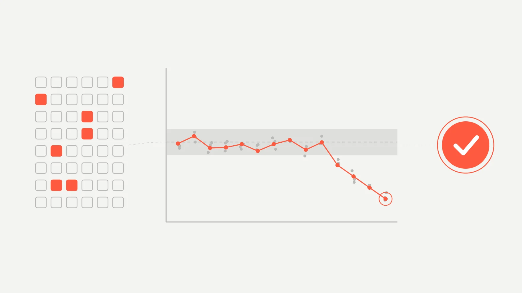
Inputs and outputs are monitored differently. On the input side, compare this week's traffic against the distribution your golden set was built from, using the same strata. A population stability index is a simple, common choice for categorical attributes:
import numpy as np
from scipy.stats import ks_2samp

def psi(expected: dict[str, float], actual: dict[str, float], eps: float = 1e-4) -> float:
    keys = sorted(expected.keys() | actual.keys())
    e = np.array([max(expected.get(k, 0.0), eps) for k in keys])
    a = np.array([max(actual.get(k, 0.0), eps) for k in keys])
    return float(np.sum((a - e) * np.log(a / e)))

# categorical: how traffic is spread across strata
stratum_shift = psi(golden.production_share, share_by_stratum(this_week))

# numeric: has the distribution of lines per order moved?
lines_shift = ks_2samp(golden.lines_per_order, lines_per_order(this_week)).pvalue
A common rule of thumb reads a PSI under 0.1 as stable and over 0.25 as a real shift, but the useful threshold is the one you calibrate on your own history. For free text, the same idea works on embeddings: cluster recent inputs and watch for clusters the golden set has no cases in. Research on detecting dataset shift suggests that simple two-sample tests on a reduced representation of the inputs work well.[6]
On the output side, the monitors are the checks you already have, run on a sample of live traffic:
- Property violation rate. The guardrails from 104 already run in production. A rising rate is the earliest signal you'll get.
- Judge pass rate on a small daily sample, scored by the calibrated judge.
- Escalation rate and correction rate. How often the agent hands a case to a person, and how often a person changes what it wrote.
When any of these move, the response is the same loop: sample the new traffic, label it, add it to the golden set in its proper stratum, recompute the production shares and rerun the baseline. Drift monitoring isn't a separate system from evaluation. It's how the golden set stays a picture of production rather than a picture of last quarter.
None of this is new to ML teams. Google's well-known rubric for production readiness lists data tests, model tests and monitoring tests side by side,[7] and the warning that ML systems pile up hidden technical debt in their data dependencies and feedback loops is more than a decade old.[8] What's new is that every team putting an agent into an operational process now has an ML system, whether or not they have an ML team.
Where it runs
| When | What runs | Against |
|---|---|---|
| Every pull request | Properties on recorded outputs; a small live golden subset | The production baseline |
| Nightly | The full golden set, pass^3, with the judge | The production baseline, with the noise margin |
| Model or prompt change | The full golden set, plus the judge's own calibration set | The production baseline |
| Weekly | Input drift, output monitors, a fresh labelled sample | The golden set's production shares |
A practical starting point
- Write down the trivial baseline and the current production score before changing anything.
- Measure the noise floor by scoring the same version three times.
- Build a golden set of 100 to 300 cases from production samples, incidents and human corrections, tagged by stratum and source, with a held-out slice nobody tunes against.
- Fill the rare strata with synthetic cases generated from structured seeds, allocated in production proportions with a floor, verified, and reported with production weights.
- Score structured fields exactly, run the 104 properties everywhere, and use a calibrated judge only for free text.
- Gate releases on pass^k against the baseline, per case and in aggregate.
- Monitor inputs and outputs weekly, and feed what drifts back into the golden set.
What's next in this series
Six posts in, we have every kind of check an agent can't talk its way around: properties, mutation scores, real databases and golden datasets with baselines. The next post brings them together around the question this series keeps returning to: how to set up a coding agent's loop so it can't grade its own homework. After that come two threads we've promised along the way, contract tests for the systems you can't put in a container, and what flaky tests cost when an agent runs your suite a hundred times a day.
If you've built a golden dataset that stayed useful for more than a quarter, tell us how. It's the hardest part of this to get right.
The testing series
- Testing 101 for the Age of Coding Agents
- Testing 102: Fast unit tests, honest end-to-end tests
- Testing 103: Mutation testing with fermut
- Testing 104: Property-based testing with Hypothesis
- Testing 105: Integration testing with Testcontainers and DuckDB
- Testing 106: Evals with baselines, golden datasets and LLM judges (this post)
References
- L. Zheng et al., "Judging LLM-as-a-Judge with MT-Bench and Chatbot Arena," NeurIPS 2023 Datasets and Benchmarks. arxiv.org/abs/2306.05685
- S. Shankar, J. D. Zamfrescu-Pereira, B. Hartmann, A. G. Parameswaran, I. Arawjo, "Who Validates the Validators? Aligning LLM-Assisted Evaluation of LLM Outputs with Human Preferences," UIST 2024. arxiv.org/abs/2404.12272
- S. Yao, N. Shinn, P. Razavi, K. Narasimhan, "τ-bench: A Benchmark for Tool-Agent-User Interaction in Real-World Domains," 2024. arxiv.org/abs/2406.12045
- J. Gama, I. Žliobaitė, A. Bifet, M. Pechenizkiy, A. Bouchachia, "A Survey on Concept Drift Adaptation," ACM Computing Surveys, 2014. doi.org/10.1145/2523813
- L. Chen, M. Zaharia, J. Zou, "How Is ChatGPT's Behavior Changing over Time?," Harvard Data Science Review, 2024. arxiv.org/abs/2307.09009
- S. Rabanser, S. Günnemann, Z. C. Lipton, "Failing Loudly: An Empirical Study of Methods for Detecting Dataset Shift," NeurIPS 2019. arxiv.org/abs/1810.11953
- E. Breck, S. Cai, E. Nielsen, M. Salib, D. Sculley, "The ML Test Score: A Rubric for ML Production Readiness and Technical Debt Reduction," IEEE Big Data 2017. research.google/pubs/the-ml-test-score
- D. Sculley et al., "Hidden Technical Debt in Machine Learning Systems," NeurIPS 2015. papers.nips.cc